DT1-Glied
Inhalt
DT1-Glied
Differenzierer mit Realisierungterm (DT\(_1\)–Glied)
\[G(s) = \frac{V_D s}{1+T_R s}\]
Diagramme in Control
import control
import numpy as np
import matplotlib.pyplot as plt
plt.style.use('ggplot')
s = control.TransferFunction.s
Vd = 10
Tr = 1/10
Gs = Vd*s/(1+Tr*s)
Gs
\[\frac{10 s}{0.1 s + 1}\]
def check_proper_tf(Gs):
    """check if transferfunction is proper"""
    return len(Gs.num[0][0]) <= len(Gs.den[0][0])

check_proper_tf(Gs)
True
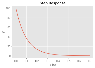
# step response
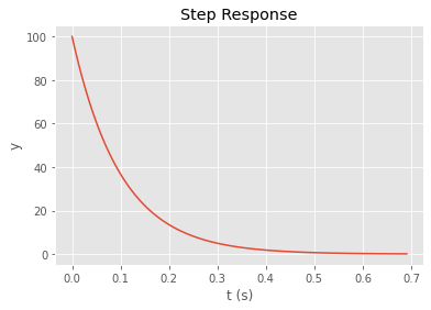
(tout, yout) = control.step_response(Gs)
plt.plot(tout,yout)
plt.title("Step Response")
plt.ylabel("y")
plt.xlabel("t (s)")
Text(0.5, 0, 't (s)')
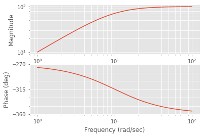
# bode diagram
fig2 = plt.figure()
(mag, phase_rad, w) = control.bode_plot(Gs)
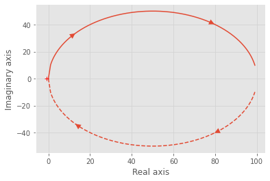
# nyquist plot
res_nyquist = control.nyquist_plot(Gs)
# pole zero map
poles, zeros = control.pzmap(Gs, plot=True)
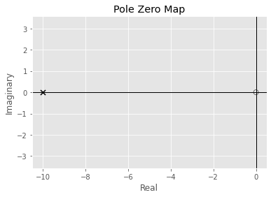
Diagramme in SciPy¶¶
import scipy.signal as signal
sys_tf = signal.TransferFunction([Vd, 0], [Tr, 1])
tout, yout = signal.step(sys_tf)
plt.plot(tout,yout)
plt.title("Step Response")
plt.ylabel("y")
plt.xlabel("t (s)")
Text(0.5, 0, 't (s)')
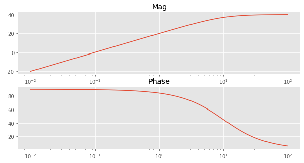
w, mag, phase = signal.bode(sys_tf)
plt.figure(figsize=(10,5))
plt.subplot(211)
plt.semilogx(w, mag)
plt.title('Mag')
plt.subplot(212)
plt.semilogx(w, phase)
plt.title('Phase')
Text(0.5, 1.0, 'Phase')
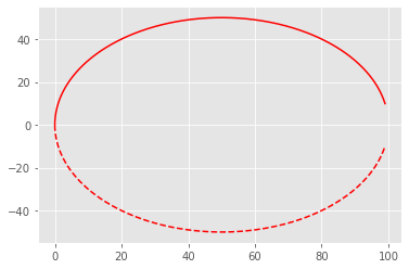
w, H = signal.freqresp(sys_tf)
plt.plot(H.real, H.imag, "r")
plt.plot(H.real, -H.imag, "r--")
[<matplotlib.lines.Line2D at 0x7f50d2792ee0>]
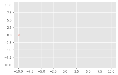
zeros, poles, k = signal.tf2zpk(sys_tf.num, sys_tf.den)
plt.plot(poles.real,poles.imag,'x',markersize=5)
plt.vlines(x=0,ymin=-10,ymax=10,linewidth=0.5,color='black')
plt.hlines(y=0,xmin=-10,xmax=10,linewidth=0.5,color='black')
<matplotlib.collections.LineCollection at 0x7f50d270ca90>