ERA - Masse Feder System
Inhalt
ERA - Masse Feder System
Die Experimentelle Modellbildung (aka Black-Box Systemidentifikation*) hat innerhalb der Ingenieurwissenschaften und der Regelungstheorie eine lange Tradition. Erste wissenschaftliche Aufsätze gehen auf die späten 1950er und frühen 1960er Jahre zurück.
Ähnliche Techniken sind derzeit innerhalb der künstlichen Intelligenz Forschung sehr beliebt. Im Englischen spricht man dann oft von Machine Learning oder Data Driven Modelling.
HoKalman / ERA
Ho und Kalman haben 1966 ihren Algorithmus vorgestellt. Die HoKalman Methode erlaubt das Lernen/Identifizieren von linearen zeitinvarianten Systemen (engl. LTI) direkt aus Messdaten. Kung hat 1978 diese Methode für den verrauschten Fall angepasst. Die moderne Version wurde 1985 von J.N. Juang und R. S. Pappa am NASA Langley Research Center vorgestellt. Ähnliche Versionen werden z.B von Luft- und Raumfahrtagenturen oder Autohersteller eingesetzt. Noch heute wird diese Methode innerhalb der Kontrolltheorie und dem maschinellen Lernen in wissenschaftlichen Aufsätzen untersucht.
Betrachten wir ein lineares zeitdiskretes System
mit den Signaldimensionen
\(\mathbf{x}_k \in \mathbb{R}^{n}, \mathbf{u}_k \in \mathbb{R}^{p}, \mathbf{y}_k \in \mathbb{R}^{q}\)
und den Matrizen mit den Dimensionen
\(\mathbf{A} \in \mathbb{R}^{n \times n}, \mathbf{B} \in \mathbb{R}^{n \times p}, \mathbf{C} \in \mathbb{R}^{q \times n}, \mathbf{D} \in \mathbb{R}^{q \times p}.\)
Für die ERA/HoKalman Methode benötigen wir Messdaten welche von einer Impulsantwort stammen. Den Eingangsimpulse wollen wir mit
kennzeichnen und die Impulsantwort mit
Markov-Parameter / Impulsantwort
Als Nächstes wollen wir die Markov-Parameter bzw. die Impulsantwort verstehen.
Dazu setzen wir in die Ausgangsgleichung
die zeitverschobene Zustandsgleichung
ein. Damit erhalten wir eine Ausgangsgleichung welche statt \(\mathbf{x}_k\) und \(\mathbf{u}_k\)
von \(\mathbf{x}_{k-1}\), \(\mathbf{u}_{k-1}\) und \(\mathbf{u}_k\) abhängig ist. Wiederholtes anwenden führt auf eine Ausgangsgleichung welche nur noch von \(\mathbf{x}_0\) und \(\mathbf{u}_k,\mathbf{u}_{k-1},\dots,\mathbf{u}_0\) abhängt.
Um diese Erkenntnis noch mal zu unterstreichen wiederholen wir dieses Vorgehen
wobei wir \(\mathbf{x}_0=\mathbf{0}\) angenommen haben.
Die Ausgangsgleichung
ergibt sich also durch eine Faltung der Markov-Parameter / (theoretische) Impulsantwort mit dem Eingang. Ist die Impulsantwort durch Daten gegeben wollen wir folgende Notation verwenden:
Diese Faltung können wir auch kurz mit
anschreiben.
Steuerbarkeit und Beobachtbarkeit
Für die ERA/HoKalman benötigen wir die Konzepte der erweiterten Steuerbarkeits- und Beobachtbarkeitsmatrizen. Aus der linearen Kontrolltheorie kennen wir die Steuerbarkeitsmatrix
Die erweiterte Steuerbarkeitsmatrix
ist prinzipiell ähnlich aufgebaut, jedoch gilt immer \(m_c > n\). In der Praxis besitzt die erweiterte Steuerbarkeitsmatrix eine deutlich größere Dimension \(m_c >> n\) als die Steuerbarkeitsmatrix.
Die gleichen Überlegungen gelten für die Beobachtbarkeitsmatrix
und für die erweiterte Beobachtbarkeitsmatrix
wobei wieder \(m_o>>n\) gilt.
Diese Matrizen sind in vielen Methoden Systemidentifikation anzutreffen.
Block Hankel Matrizen
Zentral für viele Systemidentifikationsmethoden ist die sogenannte Block Hankel Matrix. Diese Matrix
wird durch die Impulsantwort konstruiert. Die Impulsantwort wird in die erste Zeile geschrieben und dann um einen Zeitschritt versetzt in die Zweite, und so weiter und so fort.
Weiters gelten die Beziehungen
und
wobei die Vektoren wie folgt konstruiert
sind. Die Hankel Matrix verbindet alle vergangenen Eingänge mit allen zukünftigen Ausgängen. Die Matrix \(\mathbf{T}\) ist eine beliebige unitäre Transformationsmatrix.
In der Praxis operieren wir immer mit einer endlichen Anzahl von Messdaten
Durch das Einsetzen der Markov-Parameter in die Hankel Matrix
können wir die Beziehung \(\mathbf{H}_{m_o,m_c} = \boldsymbol{\mathcal{O}}_{m_o} \boldsymbol{\mathcal{C}}_{m_c}\) leicht erkennen. Diese Zerlegung erfolgt mittels einer Singulärwertzerlegung \(\boldsymbol{\mathcal{O}}_{m_o} \boldsymbol{\mathcal{C}}_{m_c}=SVD(\mathbf{H}_{m_o,m_c})\) der Hankel Matrix.
Sind die beiden Matrizen \(\boldsymbol{\mathcal{O}}_{m_o}\) und \(\boldsymbol{\mathcal{C}}_{m_c}\) vorhanden so können die Matrizen \(\color{red}{\mathbf{C}}\) und \(\color{red}{\mathbf{B}}\) leicht selektiert werden, weil die Eingangs- und Ausgangsdimensionen bekannt sind.
Für die Rekonstruktion \(\color{red}{\mathbf{A}}\) von benötigen wir eine weiter Hankel Matrix
welche jedoch um einen Zeitschritt verschoben ist. Dadurch gewinnen wir die Beziehung \(\mathbf{H}^{'}_{m_o,m_c} = \boldsymbol{\mathcal{O}}_{m_o}\color{red}{\mathbf{A}}\boldsymbol{\mathcal{C}}_{m_c}\).
Durch die Verwendung der Moore-Penrose-Inverse erfolgt ein Umstellen der obigen Gleichung auf \(\color{red}{\mathbf{A}} = \boldsymbol{\mathcal{O}}_{m_o}^{\dagger}\mathbf{H}^{'}_{m_o,m_c} \boldsymbol{\mathcal{C}}_{m_c}^{\dagger}\) womit die Rekonstruktion von \(\color{red}{\mathbf{A}}\) gelungen ist.
Die Beziehung \(\color{red}{\mathbf{D}}=\mathbf{y}^{\delta}_0\) ist aus der Definition der Markov Parameter klar ersichtlich.
Bemerkung
Eigensystem Realization Algorithm:
Konstruieren der Hankel-Matrizen \(\mathbf{H}_{m_o,m_c}\) und \(\mathbf{H}_{m_o,m_c}^{\prime}\)
Durchführung der SVD der Hankel-Matrix
Schätzung der Matrizen aus den Daten
\[\begin{split} \begin{split} & \boldsymbol{\mathcal{O}}_{m_o} = \mathbf{U}_s \mathbf{\Sigma}_s^{1/2}\mathbf{T} \\ & \boldsymbol{\mathcal{C}}_{m_c} = \mathbf{T}^{-1} \mathbf{\Sigma}_s^{1/2} \mathbf{V}_s^T \end{split} \end{split}\]Schätzungen der Zustandsraummatrizen anhand obiger Gleichungen
\[\begin{split} \begin{split} & \mathbf{A} = \mathbf{\Sigma}_s^{-1/2}\mathbf{U}_s^{T}\mathbf{H}_{m_o,m_c}^{\prime}\mathbf{V}_s\mathbf{\Sigma}_s^{-1/2} \\ & \mathbf{B} = \boldsymbol{\mathcal{C}}_{m_c}\left(:,1:q\right) \\ & \mathbf{C} = \boldsymbol{\mathcal{O}}_{m_o}(1:p,:) \\ & \mathbf{D} = \mathbf{y}_{0}^{\delta} \end{split} \end{split}\]
Code Beispiel
In diesen Abschnitt wollen wir den Algorithmus in Python implementieren und an dem Beispiel eines Masse Feder Systems testen.
Masse Feder System (2-FG)
Gegeben ist wieder das bekannte System wobei hier nur die Positionen der Massen gemessen werden können. D.h. es kann nur ein Teil der Zustände gemessen werden. (Partially Observable Markov Decision Process (POMDP), Teilweise beobachtbarer Markov-Entscheidungsprozess)
Erstelle das System
Wir wollen ein zeitdiskretes System verwenden welches aus dem zeitkontinuierlichen System durch die scipy Methode to_discrete erstellt wird.
import numpy as np
import scipy.signal as signal
import matplotlib.pyplot as plt
m1 = 1
d1 = 0.15
c1 = 0.3

m2 = 1
d2 = 0.15
c2 = 0.3

d3 = 0.15
c3 = 0.3

A = np.array([[0., 0., 1., 0.],
              [0., 0., 0., 1.],
              [-(c1+c2)/m1, c2/m1, -(d1+d2)/m1, d2/m1],
              [c2/m2, -(c2+c3)/m2, (d2)/m2, -(d2+d3)/m2]])
B = np.array([[0., 0.], [0., 0.], [1./m1, 0.], [0., 1/m2]])
C = np.array([[1., 0., 0., 0], [0., 1., 0., 0.]])
D = np.array([[0., 0.],[0., 0.]])
C
array([[1., 0., 0., 0.],
       [0., 1., 0., 0.]])
sys_c = signal.StateSpace(A, B, C, D)
print(sys_c)
StateSpaceContinuous(
array([[ 0.  ,  0.  ,  1.  ,  0.  ],
       [ 0.  ,  0.  ,  0.  ,  1.  ],
       [-0.6 ,  0.3 , -0.3 ,  0.15],
       [ 0.3 , -0.6 ,  0.15, -0.3 ]]),
array([[0., 0.],
       [0., 0.],
       [1., 0.],
       [0., 1.]]),
array([[1., 0., 0., 0.],
       [0., 1., 0., 0.]]),
array([[0., 0.],
       [0., 0.]]),
dt: None
)
eig_values, _ = np.linalg.eig(sys_c.A)
eig_values
array([-0.225+0.92161543j, -0.225-0.92161543j, -0.075+0.54256336j,
       -0.075-0.54256336j])
dt = 0.1
sys_d = sys_c.to_discrete(dt)
print(sys_d)
StateSpaceDiscrete(
array([[ 9.97038953e-01,  1.46889167e-03,  9.84204432e-02,
         7.83673580e-04],
       [ 1.46889167e-03,  9.97038953e-01,  7.83673580e-04,
         9.84204432e-02],
       [-5.88171638e-02,  2.90559288e-02,  9.67630371e-01,
         1.59968561e-02],
       [ 2.90559288e-02, -5.88171638e-02,  1.59968561e-02,
         9.67630371e-01]]),
array([[4.94800256e-03, 2.58485012e-05],
       [2.58485012e-05, 4.94800256e-03],
       [9.84204432e-02, 7.83673580e-04],
       [7.83673580e-04, 9.84204432e-02]]),
array([[1., 0., 0., 0.],
       [0., 1., 0., 0.]]),
array([[0., 0.],
       [0., 0.]]),
dt: 0.1
)
eig_values, _ = np.linalg.eig(sys_d.A)
eig_values
array([0.97360179+0.08998355j, 0.97360179-0.08998355j,
       0.99106754+0.05382452j, 0.99106754-0.05382452j])
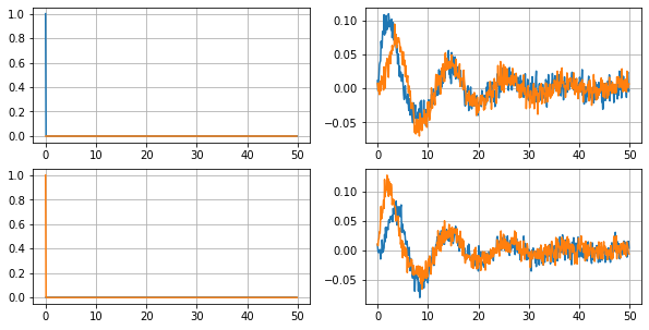
Erzeuge Messdaten für ERA
Wie theoretisch besprochen, benötigen wir eine Impulsantwort des Systems. In der Praxis werden die Impulsantworten für jeden Eingang separat erfasst und dann gestapelt.
Weiters überlagern wir die Impulsantwort mit einem Messrauschen.
t = np.arange(0,50,dt)
print(t.shape)
(500,)
u1 = np.zeros((len(t),2))
print(u1.shape)
u1[0,0] = 1
print(u1[:6,:])

u2 = np.zeros((len(t),2))
print(u2.shape)
u2[0,1] = 1
print(u2[:6,:])
(500, 2)
[[1. 0.]
 [0. 0.]
 [0. 0.]
 [0. 0.]
 [0. 0.]
 [0. 0.]]
(500, 2)
[[0. 1.]
 [0. 0.]
 [0. 0.]
 [0. 0.]
 [0. 0.]
 [0. 0.]]
tout1, yout1_, xout1 = signal.dlsim(sys_d,u1)
print(yout1_.shape)

tout2, yout2_, xout2 = signal.dlsim(sys_d,u2)
print(yout2_.shape)
(500, 2)
(500, 2)
yout1 = yout1_ + np.random.randn(len(yout1_),2)*0.01
yout2 = yout2_ + np.random.randn(len(yout2_),2)*0.01
fig = plt.figure(figsize=(10, 5))

plt.subplot(2,2,1)
plt.plot(tout1,u1)
plt.grid()

plt.subplot(2,2,2)
plt.plot(tout1,yout1)
plt.grid()

plt.subplot(2,2,3)
plt.plot(tout1,u2)
plt.grid()

plt.subplot(2,2,4)
plt.plot(tout2,yout2)
plt.grid()
yout = np.stack((yout1,yout2))
yout.shape
(2, 500, 2)
YY = yout.transpose(2,0,1)
YY.shape
(2, 2, 500)
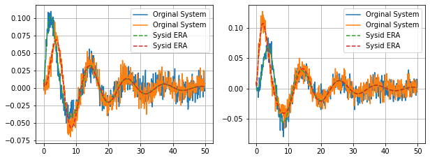
Systemidentifizierung mittels ERA
def BlockHankel(Y, mo, mc):

    nr, nc, L = Y.shape

    H = np.zeros((nr*mo,nc*mc))

    for r in range(mo):
        for c in range(mc):
            rowBeg = nr*r
            rowEnd = nr*(r+1)
            colBeg = nc*c
            colEnd = nc*(c+1)

            #print(rowBeg,rowEnd)
            #print(colBeg,colEnd)
            if (r+c<L):
                H[rowBeg:rowEnd, colBeg:colEnd] = Y[:,:,r+c]

    return H
def ERA(Y, mo, mc, r):

    nr, nc, L = Y.shape

    Hr = BlockHankel(Y[:,:,1:], mo, mc)
    Hr_p = BlockHankel(Y[:,:,2:], mo, mc)

    nx = np.linalg.matrix_rank(Hr)

    U,S,Vh = np.linalg.svd(Hr, True)
    S_mat = np.diag(S)
    Sigma = S_mat[0:r,0:r]
    Ur =U[:,0:r]
    Vhr =Vh[0:r,:]

    Sigma_inv = np.linalg.inv(Sigma)

    Ar = Sigma_inv**(0.5) @ Ur.T @ Hr_p @ Vhr.T @ Sigma_inv**(0.5)
    Br = Sigma_inv**(0.5) @ Ur.T @ Hr[:,0:nr]
    Cr = Hr[0:nc,:] @ Vhr.T @ Sigma_inv**(0.5)

    Dr = Y[:,:,0]

    HSVs = S

    return Ar, Br, Cr, Dr, HSVs, nx
r = 4
Ar, Br, Cr, Dr, HSVs, nx = ERA(YY,mo=100,mc=100,r=r)
nx
200
sysr = signal.StateSpace(Ar,Br,Cr,Dr,dt=dt)
print(sysr)
StateSpaceDiscrete(
array([[ 9.90596372e-01,  5.41136505e-02,  8.04812446e-04,
         6.29245067e-04],
       [-5.41254292e-02,  9.91365664e-01, -1.18051982e-03,
        -1.22550639e-03],
       [-1.26784150e-03, -1.12264851e-03,  9.79708374e-01,
         8.95006660e-02],
       [-3.07530892e-04,  7.77785959e-04, -8.95483693e-02,
         9.66642986e-01]]),
array([[ 0.21456143,  0.22054022],
       [ 0.21562074,  0.2121428 ],
       [-0.15103836,  0.1746997 ],
       [-0.15850599,  0.15819699]]),
array([[ 0.21590535, -0.20778459, -0.17197816,  0.15145799],
       [ 0.21912918, -0.21986231,  0.15552216, -0.16481435]]),
array([[0.01162235, 0.01012659],
       [0.00740089, 0.01118258]]),
dt: 0.1
)
tout1_simr,yout1_simr, xout1_simr = signal.dlsim(sysr,u1)
tout2_simr,yout2_simr, xout2_simr = signal.dlsim(sysr,u2)
fig = plt.figure(figsize=(10, 8))

plt.subplot(2,2,1)
plt.plot(tout1,yout1,label='Orginal System')
plt.plot(tout1_simr,yout1_simr,linestyle='--',label='Sysid ERA')
plt.grid()
plt.legend()

plt.subplot(2,2,2)
plt.plot(tout2,yout2,label='Orginal System')
plt.plot(tout2_simr,yout2_simr,linestyle='--',label='Sysid ERA')
plt.grid()
plt.legend()
<matplotlib.legend.Legend at 0x7f339c416580>
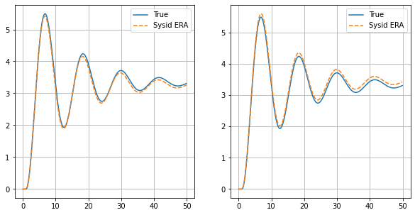
Validierung
Eine in der Praxis übliche Methode der Validierung verlangt neue Messdaten zu sammeln, welche nicht für das Identifizieren des Systems benutzt wurden. Oft genügen 2 neue Signale. Hier verwenden wir einen sin und einen step. Der Vorteil dieser Methode ist, dass die identifizierten Modelle sehr gut generalisieren müssen um diesen Test zu bestehen.
Sowohl das Feld der Systemidentifikation als auch das Feld des Maschinellen Lernens beinhalten weitere Theorien und Methoden wie man die Güte eines gelernten Systems validiert.
Validierung 1
u = sin(t)
t_sim = np.arange(0,50,dt)
print(t_sim.shape)
(500,)
u1 = np.zeros((len(t_sim),2))
u1[:,0] = np.sin(t_sim)
tout1, yout1, xout1 =signal.dlsim(sys_d,u1)
tout1_simr,yout1_simr, xout1_simr = signal.dlsim(sysr,u1)
plt.subplots(1, 1, figsize = (10, 5))
plt.subplot(1,2,1)
plt.plot(tout1,yout1[:,0],label='True')
plt.plot(tout1_simr,yout1_simr[:,0],linestyle='--',label='Sysid ERA')
plt.grid()
plt.legend()
plt.subplot(1,2,2)
plt.plot(tout1,yout1[:,1],label='True')
plt.plot(tout1_simr,yout1_simr[:,1],linestyle='--',label='Sysid ERA')
plt.grid()
plt.legend()
<matplotlib.legend.Legend at 0x7f339c291580>
Validierung 2
u = step(t)
u1 = np.ones((len(t_sim),2))
u1.shape
(500, 2)
# Input sequence
u1 = np.ones((len(t_sim),2))
u1[:10,:] = 0
tout1, yout1, xout1 =signal.dlsim(sys_d,u1)
tout1_simr,yout1_simr, xout1_simr = signal.dlsim(sysr,u1)
plt.subplots(1, 1, figsize = (10, 5))
plt.subplot(1,2,1)
plt.plot(tout1,yout1[:,0],label='True')
plt.plot(tout1_simr,yout1_simr[:,0],linestyle='--',label='Sysid ERA')
plt.grid()
plt.legend()
plt.subplot(1,2,2)
plt.plot(tout1,yout1[:,1],label='True')
plt.plot(tout1_simr,yout1_simr[:,1],linestyle='--',label='Sysid ERA')
plt.grid()
plt.legend()
<matplotlib.legend.Legend at 0x7f339a962a90>
Fazit
Wir haben eine experimentelle Modellbildung mit der Hilfe der HoKalman/ERA Methode durchgeführt. Dadurch ist es uns gelungen ein Modell \(\left(\color{red}{\mathbf{A}},\color{red}{\mathbf{B}},\color{red}{\mathbf{C}},\color{red}{\mathbf{D}}\right)\) direkt aus Messdaten zu identifizieren.
Referenzen
The rise of data-driven modelling, Nature Reviews Physics, June 2021
Samet Oymak and Necmiye Ozay, „Non-asymptotic identification of lti systems from a single trajectory“, 2019 American control conference (ACC), 2019.