Scipy¶

Hier wollen wir nun die Bibliothek SciPy kennen lernen. SciPy baut auf NumPy auf und beinhaltete eine Menge Werkzeuge für die Wissenschaftliche Programmierung:

Signalverarbeitung (scipy.signal)
Lineare Algebra (scipy.linalg)
Nummerische Integration (scipy.integrate)
Interpolation (scipy.interpolate)
Optimierung (scipy.optimize)
Fouier Transfomation (scipy.fft)
Statistik (scipy.stats)
etc (vieles mehr)

Wir werden hier nur ein paar Beispiele besprechen. Ein vollständiges Kennenlernen von SciPy würde ganze Bücher füllen und wahrscheinlich Monate, wenn nicht Jahre benötigen.

Signale und System in SciPy¶

Als erstes wollen wir uns das Submodul scipy.signal ansehen. Konkret starten wir mit LTI Systemen die vor allem für die Signalverarbeitung aber auch für die Regelungstechnik geeignet ist.

LTI¶

Gegeben sei ein 1 Massenschwinger mit

\[\begin{split} \begin{bmatrix} \dot{x}_1 \\ \dot{x}_2 \end{bmatrix} = \begin{bmatrix} 0 & 1 \\ -\frac{c}{m} & -\frac{d}{m} \end{bmatrix} \begin{bmatrix} x_1 \\ x_2 \end{bmatrix} + \begin{bmatrix} 0 \\ \frac{1}{m} \end{bmatrix} u \end{split}\]

from scipy import signal
import numpy as np
import matplotlib.pyplot as plt
plt.style.use('ggplot')

m = 1; d = 0.2; c = 0.5

A = np.array([[0, 1], [-c/m,-d/m]])
B = np.array([[0], [1]])
C = np.array([[1, 0]])
D = np.zeros((1,1))

sys = signal.StateSpace(A,B,C,D)
sys

StateSpaceContinuous(
array([[ 0. ,  1. ],
       [-0.5, -0.2]]),
array([[0],
       [1]]),
array([[1, 0]]),
array([[0.]]),
dt: None
)

sys.B.shape

(2, 1)

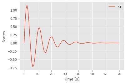
t, y = signal.impulse(sys)
plt.plot(t,y)
plt.legend([r'$x_1$'])
plt.xlabel('Time [s]')
plt.ylabel('States')

Text(0, 0.5, 'States')

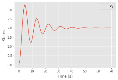
t, y = signal.step(sys)
plt.plot(t,y)
plt.legend([r'$x_1$'])
plt.xlabel('Time [s]')
plt.ylabel('States')

Text(0, 0.5, 'States')

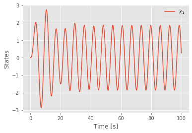
t = np.linspace(0,100,1000)
u = np.sin(t)

tout, yout, xout = signal.lsim(sys, U=u, T=t)
plt.plot(tout,yout)
plt.legend([r'$x_1$'])
plt.xlabel('Time [s]')
plt.ylabel('States')

Text(0, 0.5, 'States')

tf = signal.TransferFunction(sys)

/home/johannes/miniconda3/envs/python-beginners2/lib/python3.9/site-packages/scipy/signal/filter_design.py:1631: BadCoefficients: Badly conditioned filter coefficients (numerator): the results may be meaningless
  warnings.warn("Badly conditioned filter coefficients (numerator): the "

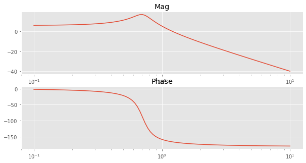
w, mag, phase = signal.bode(sys)

plt.figure(figsize=(10,5))
plt.subplot(211)
plt.semilogx(w, mag)
plt.title('Mag')
plt.subplot(212)
plt.semilogx(w, phase)
plt.title('Phase')

Text(0.5, 1.0, 'Phase')

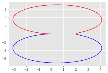
w, H = signal.freqresp(sys)

/home/johannes/miniconda3/envs/python-beginners2/lib/python3.9/site-packages/scipy/signal/filter_design.py:1631: BadCoefficients: Badly conditioned filter coefficients (numerator): the results may be meaningless
  warnings.warn("Badly conditioned filter coefficients (numerator): the "

plt.plot(H.real, H.imag, "b")
plt.plot(H.real, -H.imag, "r")

[<matplotlib.lines.Line2D at 0x7fe37284d2e0>]

sysd = sys.to_discrete(dt=0.1)

Linear Algebra in SciPy¶¶

Das Submodul scipy.linalg baut auf numpy.linalg auf und importiert dies Funktion meist mit dem gleichen Namen.

from scipy import linalg

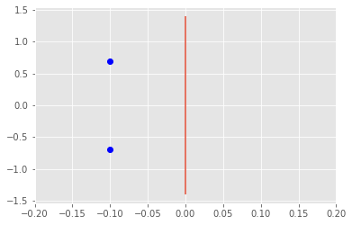
eigvals = linalg.eigvals(sys.A)

vmax = np.max(np.abs(np.imag(eigvals)))*2
hmax = np.max(np.abs(np.real(eigvals)))*2
plt.figure()
plt.plot(np.real(eigvals),np.imag(eigvals),'o',c='blue')
plt.vlines(0,ymin=-vmax,ymax=vmax)
plt.xlim([-hmax,hmax]);

Optimierung in Scipy¶

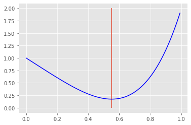
Minimierung einer Funktion mit einer Variablen¶

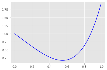
from scipy.optimize import minimize_scalar

def objective_function(x):
    return 3 * x ** 4 - 2 * x + 1

x = np.arange(0,1,0.01)
y = objective_function(x)

plt.plot(x,y,c='blue')

[<matplotlib.lines.Line2D at 0x7fe370d16400>]

res = minimize_scalar(objective_function)
res

     fun: 0.17451818777634331
    nfev: 16
     nit: 12
 success: True
       x: 0.5503212087491959

plt.plot(x,y,c="blue")
plt.vlines(res.x,ymin=0,ymax=2)

<matplotlib.collections.LineCollection at 0x7fe370fdbee0>

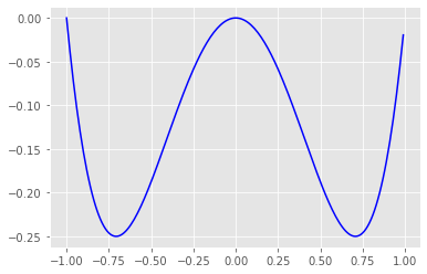
def objective_function(x):
    return x ** 4 - x ** 2

x = np.arange(-1,1,0.01)
y = objective_function(x)

plt.plot(x,y,c='blue')

[<matplotlib.lines.Line2D at 0x7fe371499730>]

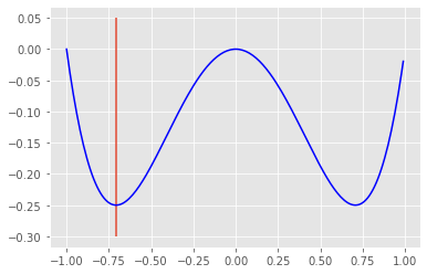
res = minimize_scalar(objective_function,  method='bounded', bounds=(-1, 0))
res

     fun: -0.24999999999998732
 message: 'Solution found.'
    nfev: 10
  status: 0
 success: True
       x: -0.707106701474177

plt.plot(x,y,c="blue")
plt.vlines(res.x,ymin=-0.30,ymax=0.05)

<matplotlib.collections.LineCollection at 0x7fe370bc5190>

Fouier Transfomation in SciPy¶

Scipy bietet viele Methoden für die Fourier-Analyse. Wir wollen hier ein Beispiel besprechen, wie es oft in einem Ingenieurstudium gezeigt wird. Ziel ist es ein Signal vom Rauschen zu trennen. Dazu wird das Signal in den Frequenzbereich transformiert, dort analysiert und vom Rauschen getrennt. Schlussendlich soll das Signal rekonstruiert werden.

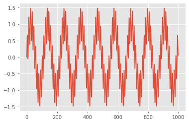
Generierung Signalen¶

from scipy.fft import fft, fftfreq

def generate_sine_wave(freq, sample_rate, duration):
    x = np.linspace(0, duration, sample_rate * duration, endpoint=False)
    frequencies = x * freq
    # 2pi because np.sin takes radians
    y = np.sin((2 * np.pi) * frequencies)
    return x, y

sample_rate = 44100  # hertz
duration = 5  # seconds

_, sin_signal = generate_sine_wave(400, sample_rate, duration)
_, sin_noise = generate_sine_wave(4000, sample_rate, duration)


signal = sin_signal + sin_noise*0.5

plt.plot(signal[:1000])
plt.show()

Wir haben also

FFT - Fast Fourier Transformation¶

# Number of samples in normalized_tone
N = sample_rate * duration

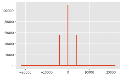
yf = fft(signal)
xf = fftfreq(N, 1 / sample_rate)

plt.plot(xf, np.abs(yf))
plt.show()

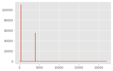
from scipy.fft import rfft, rfftfreq

# Note the extra 'r' at the front
yf = rfft(signal)
xf = rfftfreq(N, 1 / SAMPLE_RATE)

plt.plot(xf, np.abs(yf))
plt.show()

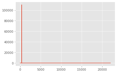
# The maximum frequency is half the sample rate
points_per_freq = len(xf) / (SAMPLE_RATE / 2)

# Our target frequency is 4000 Hz
target_idx = int(points_per_freq * 4000)

yf[target_idx - 1 : target_idx + 2] = 0

plt.plot(xf, np.abs(yf))
plt.show()

Anwenden der inversen FFT¶

from scipy.fft import irfft

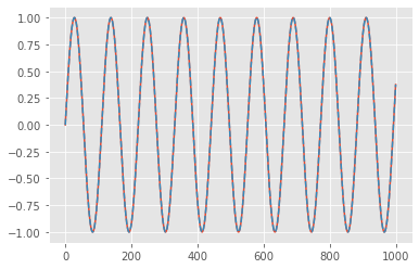
new_sig = irfft(yf)

plt.plot(new_sig[:1000])
plt.plot(sin_signal[:1000],'--')
plt.show()

Python für die Kybernetik

Scipy

Inhalt